# Load necessary libraries
library(matrixStats)
library(factoextra)
library(ggplot2)
library(gplots)
library(RColorBrewer)
library(limma)
library(gridExtra)
library(ggsci)
library(EnhancedVolcano)
library(UpSetR)
library(eulerr)
library(pheatmap)
library(KEGGREST)
library(clusterProfiler)
library(org.Mmu.eg.db)
library(dplyr)

# Set up standard input/output locations used throughout the analysis.
data_dir <- "data"
results_dir <- paste0("results/", Sys.Date())
dir.create(results_dir, recursive = TRUE)
knitr::opts_chunk$set(seed = 1)

# Load expression matrix, sample metadata, probe QC flags, and probe annotation.
MA <- read.csv(file.path(data_dir, "MAdata.csv"), header = TRUE, row.names = 1, check.names = FALSE)
MAinfo <- read.csv(file.path(data_dir, "MAinfo.csv"), header = TRUE, row.names = 1, check.names = FALSE)
ProbeBG <- read.csv(file.path(data_dir, "ProbeOverBackground.csv"), header = TRUE, row.names = 1, check.names = FALSE)
ProbeInfo <- read.csv(file.path(data_dir, "ProbeInfo.csv"), header = TRUE, row.names = 1, check.names = FALSE) %>%
  mutate("ProbeID"=rownames(.))

# Validate table alignment before analysis to avoid silent row/column mismatches.
stopifnot(identical(rownames(MA), rownames(ProbeInfo)))
stopifnot(identical(rownames(MAinfo), colnames(MA)))
stopifnot(identical(rownames(ProbeInfo), rownames(ProbeBG)))
stopifnot(identical(colnames(MA), colnames(ProbeBG)))

# Define a consistent color palette for vaccine groups across all figures.
vaccine_colors <- c(
  mRNA = "#EE2926",
  Vaxigrip = "#456990",
  Fluad = "#49BEAA"
)Influenza vaccine study
Microarray data analysis
This document provides a step-by-step guide for microarray analysis in R. Input data is read from data/, and outputs are written to a date-stamped folder under results/.
Setup
Data Preprocessing
# Work on log2 scale for downstream linear modeling.
MA <- log2(MA)

# Keep probes with valid gene annotations.
MA.clean <- MA[ProbeInfo$GeneID != 0, ]
ProbeBG <- ProbeBG[ProbeInfo$GeneID != 0, ]

# Retain probes above background in at least one sample.
ProbeBG$sum <- rowSums(ProbeBG == "TRUE")
ProbeBG <- ProbeBG[ProbeBG$sum > 0, ]

# Apply the same probe filter to the expression matrix.
MA.clean <- MA.clean[rownames(ProbeBG), ]

# Remove probes with missing expression values.
MA.clean <- MA.clean[rowSums(is.na(MA.clean)) == 0, ]

# Filter probes by variance (e.g., sd > 0.25)
#keep_var <- apply(MA.clean, 1, sd) > 0.5
#MA.clean <- MA.clean[keep_var, ]
Principal Component Analysis (PCA)
All samples 0-24h
# PCA on all retained probes to inspect global sample structure.
MA.pca <- prcomp(t(MA.clean), scale. = TRUE)
score.df <- as.data.frame(MA.pca$x)
score.df$Vaccine <- MAinfo[rownames(score.df), "Vaccine"]
score.df$Timepoint <- MAinfo[rownames(score.df), "Timepoint"]
score.df$NHP <- MAinfo[rownames(score.df), "AnimalID"]
score.df <- score.df %>% filter(!Timepoint %in% c("W4-24h", "W4-24H"))
score.df$Vaccine <- factor(score.df$Vaccine, levels = c("mRNA", "Vaxigrip", "Fluad"))

# Percent variance explained by PC1 and PC2.
var_explained <- summary(MA.pca)$importance[2, 1:2] * 100  # PC1 and PC2

# Helper to keep PCA panel styling consistent across stratifications.
pca_plot <- function(data, color_var, title) {
 p <- ggplot(data, aes(x = PC1, y = PC2, color = .data[[color_var]], shape =.data[["Timepoint"]])) +
      geom_point(size = 2) +
      theme_minimal() +
      theme(aspect.ratio = 1,
            panel.border = element_rect(color = "black",
                                      fill = NA,
                                      linewidth = 1),
            axis.text.x = element_text(size = 12),
            axis.text.y = element_text(size = 12)) +
      labs(x = paste0("PC1 (", round(var_explained[1], 1), "%)"),
           y = paste0("PC2 (", round(var_explained[2], 1), "%)"),
           title = title)
  if (color_var == "Vaccine")
    p <- p + scale_color_manual(values = vaccine_colors) + labs (title = "") else p
 return(p)
}

p1 <- pca_plot(score.df, "Vaccine", "PCA by Vaccine")
p2 <- pca_plot(score.df, "Timepoint", "PCA by Timepoint")
p3 <- pca_plot(score.df, "NHP", "PCA by NHP")

# Save multi-panel and vaccine-focused PCA figures.
ggsave(file.path(results_dir, "PCA_plots.pdf"), arrangeGrob(p1, p2, p3, ncol = 3), width = 15, height = 5)

ggsave(plot = p1, filename = file.path(results_dir, "PCA_plot_vaccine_group.pdf"), width = 4, height = 4)
Samples 24h fold change
# Pair each animal baseline (0H) with 24H for within-animal fold-change analysis.
ids <- intersect(MAinfo$AnimalID[MAinfo$Timepoint == "0H"],
                 MAinfo$AnimalID[MAinfo$Timepoint == "24H"])
s0 <- sapply(ids, function(id) rownames(MAinfo)[MAinfo$AnimalID == id & MAinfo$Timepoint == "0H"][1])
s24 <- sapply(ids, function(id) rownames(MAinfo)[MAinfo$AnimalID == id & MAinfo$Timepoint == "24H"][1])

# Compute per-probe within-animal log2 fold change (24H - 0H).
fc <- MA.clean[, s24]- MA.clean[, s0]

# PCA
pca <- prcomp(t(fc), scale. = TRUE)
var_exp <- summary(pca)$importance[2, 1:2] * 100
score.df <- data.frame(pca$x, Vaccine = MAinfo[s24, "Vaccine"])
score.df$Vaccine <- factor(score.df$Vaccine, levels = c("mRNA", "Vaxigrip", "Fluad"))


# Plot fold-change PCA with group ellipses to highlight separation.
p <- ggplot(score.df, aes(PC1, PC2, color = Vaccine, fill = Vaccine)) +
  geom_point(size = 2) +
  stat_ellipse(type = "norm", alpha = 0.2, geom = "polygon", color = NA, level = .75) +
  theme(aspect.ratio = 1,
        panel.border = element_rect(color = "black", fill = NA),
        panel.background = element_blank()) +
  labs(x = sprintf("PC1 (%.1f%%)", var_exp[1]),
       y = sprintf("PC2 (%.1f%%)", var_exp[2])) +
  scale_color_manual(values = vaccine_colors) +
  scale_fill_manual(values = vaccine_colors)

p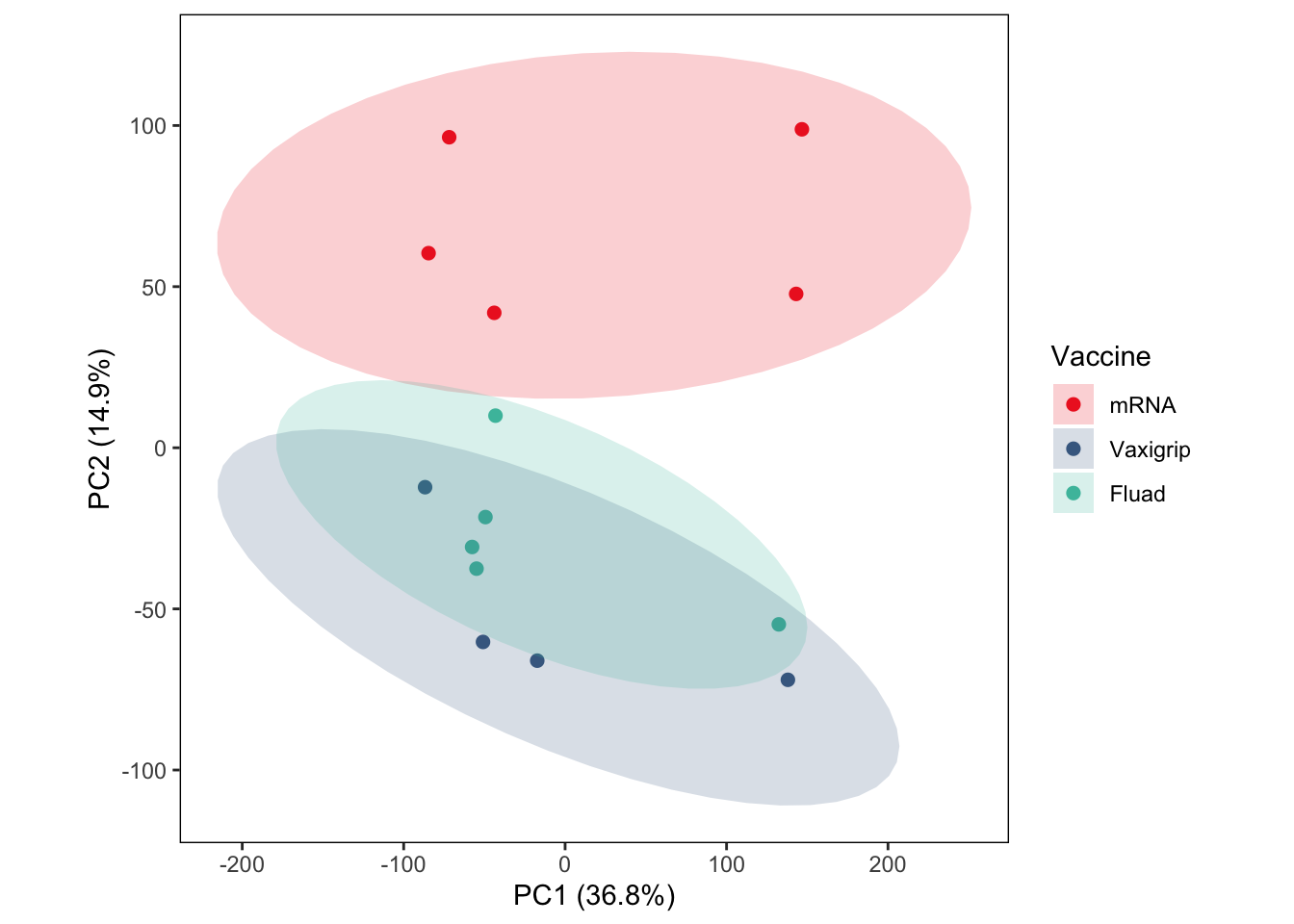
ggsave(file.path(results_dir, "PCA_log2FC_24h_vs_0h_ellipses.pdf"), p, width = 4, height = 4)Differential Expression Analysis
# Keep a single representative probe per gene (largest absolute t-statistic).
findLargest <- function(probe, gene, tstat) {
  names(tstat) <- probe
  best <- sapply(split(tstat, gene), function(x) names(which.max(abs(x))))
  best
}

# Differential expression per vaccine using paired design (AnimalID + Timepoint).
deg_analysis <- function(group) {
  samples <- rownames(MAinfo[MAinfo$Vaccine == group & MAinfo$Timepoint %in% c("0H", "24H"), ])
  design <- model.matrix(~ AnimalID + Timepoint, data = MAinfo[samples, ])
  topTable(eBayes(lmFit(MA.clean[, samples], design), trend = TRUE, robust = TRUE), coef = "Timepoint24H", number = Inf, adjust.method = "BH")
}

# Run DEG for each vaccine and collapse multiple probes to one probe per gene.
groups <- c("mRNA", "Vaxigrip", "Fluad")
deg_results <- lapply(groups, function(group) {
  deg <- deg_analysis(group)
  deg$qvalue <- qvalue::qvalue(deg$P.Value)$qvalues
  deg$ProbeID <- rownames(deg)
  deg <- left_join(deg, ProbeInfo, by = "ProbeID")
  deg <- deg[!is.na(deg$GeneID), ]
  keep <- findLargest(deg$ProbeID, deg$GeneID, deg$t)
  deg[match(keep, deg$ProbeID), ]
})
names(deg_results) <- groups

# Save results
for (g in groups) {
  write.table(deg_results[[g]], file.path(results_dir, paste0("DEG_", g, "_with_gene_symbols.tsv")),
              sep = "\t", row.names = FALSE)
}
Volcano plots
# Volcano plot per vaccine with manual coloring for up/down/non-significant probes.
for (group in names(deg_results)) {
  df <- deg_results[[group]]
  labs <- df$GeneID

  up <- df$qvalue < 0.05 & df$logFC > 1
  down <- df$qvalue < 0.05 & df$logFC < -1

  p <- EnhancedVolcano(
    df,
    lab = labs,
    selectLab = "none",
    x = 'logFC',
    y = 'P.Value',
    pCutoff = NA,
    FCcutoff = 1,
    pointSize = 1,
    colCustom = setNames(
      ifelse(up, "#f44336", ifelse(down, "#3f51b5", "grey")),
      rownames(df)
    ),
    axisLabSize = 15,
    colAlpha = 1,
    drawConnectors = TRUE,
    boxedLabels = TRUE,
    title = NULL,
    subtitle = NULL,
    caption = NULL,
    legendPosition = "none",
    xlim = c(-5, 10),
    ylim = c(0, 10)
  ) +
    theme(axis.text.x = element_text(color = "black")) +
    annotate("text", x = 9.5, y = 9.5, label = paste("Up:\n", sum(up)), hjust = 1, size = 5) +
    annotate("text", x = -5, y = 9.5, label = paste("Down:\n", sum(down)), hjust = 0, size = 5)

  ggsave(file.path(results_dir, paste0("volcano_", group, ".pdf")), p, width = 4, height = 4)
}
Differential expression with time as interaction term
Evaluate if there is any interaction between time and group. This is done to see if there is any specific changes in a group but not in the others.
# Interaction model setup: test whether time response differs by vaccine.
MAinfo$Vaccine <- relevel(factor(MAinfo$Vaccine), ref = "mRNA")
keep <- rownames(MAinfo)[MAinfo$Timepoint %in% c("0H", "24H")]
design <- model.matrix(~ AnimalID + Vaccine * Timepoint, data = MAinfo[keep, ])
fit <- eBayes(lmFit(MA.clean[, keep], design))
Coefficients not estimable: VaccineFluad VaccineVaxigrip # Reuse probe-collapsing logic after interaction-model contrasts.
filter_by_gene <- function(df) {
df$ProbeID <- rownames(df)
df <- left_join(df, ProbeInfo, by = "ProbeID")
keep <- findLargest(df$ProbeID, df$GeneID, abs(df$t))
df[match(keep, df$ProbeID), ]
}
# Extract interaction contrasts against mRNA reference and collapse probes.
mrna_vaxigrip <- filter_by_gene(
topTable(fit, coef = "VaccineVaxigrip:Timepoint24H", number = 1e6)
)
mrna_fluad <- filter_by_gene(
topTable(fit, coef = "VaccineFluad:Timepoint24H", number = 1e6)
)
# Partition interaction DEGs into group-specific and shared sets.
mrna_fluad_filtered <- mrna_fluad[!rownames(mrna_fluad) %in% rownames(mrna_vaxigrip),]
mrna_vaxigrip_filtered <- mrna_vaxigrip[!rownames(mrna_vaxigrip) %in% rownames(mrna_fluad),]
shared <- mrna_vaxigrip[rownames(mrna_vaxigrip) %in% rownames(mrna_fluad),]
#cat(paste0(ProbeInfo[rownames(mrna_fluad_filtered),]$GeneID, collapse = "\n"))Plot selected genes
# Candidate genes to visualize across vaccine/timepoint combinations.
genes_of_interest <- c("CCL2", "IFNAR1","IFNAR2", "APOBEC3A", "SCIN", "LRG1" , "LOXL1", "CCL8", "MS4A4A", "OAS1", "IL23A", "LOC699418", "LGALS17C", "LOC699418", "GSG1", "CCR3", "ISG15", "HERC5", "IFIT3","RPL35A")

for(i in seq_along(genes_of_interest)) {
  gene_to_plot <- genes_of_interest[i]
  print(gene_to_plot)
# Find representative probe for the selected gene (using mRNA DEG table).
probe_id <- deg_results[["mRNA"]]$ProbeID[deg_results[["mRNA"]]$GeneID == gene_to_plot]

# Build tidy expression table with sample annotations for plotting.
expr <- MA[probe_id, ]
df <- data.frame(
  Expression = as.numeric(expr),
  Vaccine = MAinfo[names(expr), "Vaccine"],
  Timepoint = MAinfo[names(expr), "Timepoint"],
  AnimalID = MAinfo[names(expr), "AnimalID"]
) %>% filter(!Timepoint %in% c("W4-24h", "W4-24H"))
df$Vaccine <- factor(df$Vaccine, levels = c("mRNA", "Vaxigrip", "Fluad"))

# Build ordered x-axis labels (group_timepoint) for consistent plotting.
df$VaccineTimepoint <- factor(
  paste(df$Vaccine, df$Timepoint, sep = "_"),
  levels = unique(paste(rep(c("mRNA", "Vaxigrip", "Fluad"), each = length(unique(df$Timepoint))),
                        rep(unique(df$Timepoint), times = 3), sep = "_"))
)
# Draw expression distribution and save one PDF per selected gene.
ggplot(df, aes(x = VaccineTimepoint, y = Expression, color = Vaccine)) +
  geom_boxplot(outlier.shape = "") +
  geom_jitter(width = 0.2, size = 2) +
  labs(x = "", title = gene_to_plot, y = "Normalized expression (Log2)") +
  scale_color_manual(values = vaccine_colors) +
  #ylim(0,20) +
  theme_bw() +
  theme(axis.text.x = element_text(angle = 45, hjust = 1, size = 14, color = "black"),
        aspect.ratio = 1,
        axis.text.y = element_text(size = 14, color = "black"),
        axis.title.y = element_text(size = 14))

  ggsave(file.path(results_dir, paste0("selected_genes/",gene_to_plot,"_expression" , ".pdf")), width = 4, height = 4)
}
[1] "CCL2"[1] "IFNAR1"[1] "IFNAR2"[1] "APOBEC3A"[1] "SCIN"[1] "LRG1"[1] "LOXL1"[1] "CCL8"[1] "MS4A4A"[1] "OAS1"[1] "IL23A"[1] "LOC699418"[1] "LGALS17C"[1] "LOC699418"[1] "GSG1"[1] "CCR3"[1] "ISG15"[1] "HERC5"[1] "IFIT3"[1] "RPL35A"Heatmap clusters ORA
### Adapted Heatmap with Modules and KEGG Enrichment ###


# 1) Collect significant interaction DEGs using consistent significance cutoffs.
degs_interaction <- list(mrna_vaxigrip, mrna_fluad)
all_degs <- lapply(degs_interaction, function(x) {
  x %>% filter(adj.P.Val < 0.05, abs(logFC) > 1) %>%
    dplyr::select(GeneID, logFC, adj.P.Val, ProbeID)
})

# Merge interaction DEGs and keep one entry per gene.
combined_degs <- do.call(rbind, all_degs) %>%
  group_by(GeneID) %>%
  slice_max(order_by = logFC, with_ties = FALSE) %>%
  ungroup()

# Save merged interaction DEG table.

write.csv(combined_degs, file = file.path(results_dir, "combined_DEGs_interaction.csv"), row.names = FALSE)

# 2) Build expression matrix for DEG probes and relabel rows by GeneID.
expr_matrix <- fc[rownames(fc) %in% combined_degs$ProbeID, ]
expr_matrix <- expr_matrix[!duplicated(ProbeInfo[rownames(expr_matrix), "GeneID"]), ]
rownames(expr_matrix) <- ProbeInfo[rownames(expr_matrix), "GeneID"]

# 3) Cluster DEG expression profiles into modules.
scaled_expr <- t(scale(t(expr_matrix)))

# Hierarchical clustering with Ward linkage on Euclidean distance.
gene_dist <- dist(scaled_expr, method = "euclidean")
gene_clust <- hclust(gene_dist, method = "ward.D2")

gg_color_hue <- function(n) {
  hues = seq(15, 375, length = n + 1)
  hcl(h = hues, l = 65, c = 100)[1:n]
}

modules <- cutree(gene_clust, k = 6)
module_colors <- gg_color_hue(max(modules))[modules]

# 4) Run GO enrichment for each module (background: mRNA interaction genes).
## --- 1. download & parse all Macaca pathways safely -------------

#mcc_pathways <- keggList("pathway", "mcc")
#pathway_ids  <- names(mcc_pathways)

#safe_keggGet <- function(id) tryCatch(keggGet(id)[[1]], error = \(e) NULL)

#pathway_data <- Filter(Negate(is.null), lapply(pathway_ids, safe_keggGet))

#pathway_genes <- setNames(lapply(pathway_data, \(x) {
#  g <- x$GENE
#  if (is.null(g) || length(g) < 2) return(character(0))
#  raw_entries <- g[seq(2, length(g), 2)]
# gene_symbols <- sub(";.*", "", raw_entries)
# gene_symbols[!grepl("^\\[KO:", gene_symbols)]
#}), sapply(pathway_data, `[[`, "NAME"))


#saveRDS(pathway_genes, "../data/mcc_kegg_pathways.rds")
pathway_genes <- readRDS("data/mcc_kegg_pathways.rds")

## --- 2. enrichment function -------------------------------------

# Map gene symbols to Entrez IDs
symbol_to_entrez <- function(x) unique(bitr(x, "SYMBOL", "ENTREZID", org.Mmu.eg.db)$ENTREZID)

enrichment <- function(genes, universe) enrichGO(
  gene = symbol_to_entrez(genes),
  universe = symbol_to_entrez(universe),
  ont = "BP", OrgDb = org.Mmu.eg.db,
  pAdjustMethod = "BH", qvalueCutoff = 0.05
)

module_enrichment <- setNames(lapply(unique(modules), function(m) {
  genes <- names(modules)[modules == m]
  res <- tryCatch(enrichment(genes, mrna_vaxigrip$GeneID), error = \(e) { message("Module ", m, ": ", e$message); NULL })
  if (!is.null(res) && nrow(res@result)) simplify(res, 0.8, "p.adjust", min) else res
}), paste0("M", unique(modules)))

# Prepare row/column annotations for heatmap visualization.
module_annotation <- data.frame(module = factor(modules), row.names = names(modules))
module_colors <- setNames(pal_jama()(length(unique(modules))), unique(modules))
col_order <- colnames(scaled_expr)

# Draw heatmap with module and vaccine annotations.
MAinfo_filtered <- MAinfo %>% filter(Timepoint == "24H")
stopifnot(all(rownames(MAinfo_filtered) == colnames(scaled_expr)))

pheatmap(
  scaled_expr,
  annotation_row = module_annotation,
  annotation_col = MAinfo_filtered[col_order, "Vaccine", drop = FALSE],
  cluster_rows = gene_clust,
  cutree_rows = length(unique(modules)),
  annotation_colors = list(module = module_colors, Vaccine = vaccine_colors),
  color = colorRampPalette(c("#3f51b5", "white", "#f44336"))(100),
  scale = "none", show_rownames = FALSE, show_colnames = FALSE,
  filename = file.path(results_dir, "module_heatmap_degs_interaction.pdf"),
  width = 5,
  height = 5
)
Plot GO results
df <- data.table::rbindlist(lapply(names(module_enrichment), function(m) {
  res <- module_enrichment[[m]]
  if (!is.null(res) && nrow(res@result) > 0)
    cbind(as.data.frame(res@result), module = m)
}), fill = TRUE)

top <- df[p.adjust < 0.05, head(.SD[order(p.adjust)], 3), by = module]
desired_order <- paste0("M",c(3, 5, 6, 2, 1, 4))
top$module <- factor(top$module, levels = desired_order)
top$Description <- paste0(toupper(substr(top$Description, 1, 1)), substr(top$Description, 2, nchar(top$Description)))

module_colors <- setNames(pal_jama()(length(unique(modules))), paste0("M",unique(modules)))

ggplot(top, aes(-log10(p.adjust), Description, fill = module, color = module)) +
  geom_segment(aes(x = 0, xend = -log10(p.adjust), yend = Description), size = 5) +
  geom_point(size = 6, shape = 21, color = "black", stroke = 1) +
  facet_wrap(~ module, ncol = 1, scales = "free_y") +
  geom_vline(xintercept = -log10(0.05), linetype = "dotted", color = "grey40", size = 1) +
  labs(x = "-log10(Adjusted P-value)", y = NULL) +
  scale_y_discrete(position = "right") +
  scale_color_manual(values = module_colors)+
  scale_fill_manual(values = module_colors)+
  theme_minimal() +
  theme(axis.text.y = element_text(face = "bold"),
        legend.position = "none",
        panel.grid = element_blank())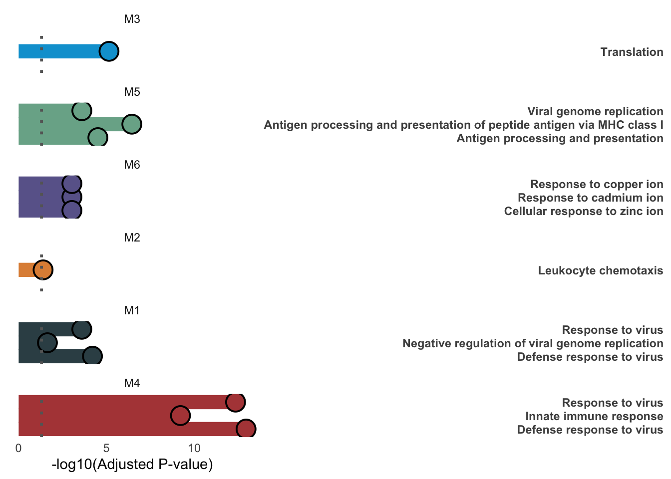
ggsave(file.path(results_dir, "modules_ORA_GO.pdf"), width = 6, height = 5)Modules over time
# 1) Select one probe per gene for module-over-time summaries.
top_probes <- bind_rows(mrna_fluad, mrna_vaxigrip) %>%
  group_by(GeneID) %>%
  slice_max(abs(logFC), n = 1, with_ties = FALSE) %>%
  filter(ProbeID %in% rownames(MA.clean), GeneID %in% names(modules)) %>%
  mutate(Module = modules[GeneID])

# 2) Convert expression matrix to tidy long format and join sample metadata.
expr_long <- MA.clean[top_probes$ProbeID, ] %>%
  as.data.frame() %>%
  tibble::rownames_to_column("ProbeID") %>%
  tidyr::pivot_longer(-ProbeID, names_to = "Sample", values_to = "Expr") %>%
  left_join(top_probes, by = "ProbeID") %>%
  mutate( Animal = stringr::str_extract(Sample, "I\\d+"),
          Time = stringr::str_replace(stringr::str_extract(Sample, "D0|24H"), "D0", "0H"),
          Time = factor(Time, levels = c("0H", "24H")),
          Vaccine = MAinfo$Vaccine[match(Animal, MAinfo$Animal)]
          ) %>%
  filter(!is.na(Time))

# 3) Average expression by module, vaccine, timepoint, and animal.
plot_df <- expr_long %>%
  group_by(Module, Vaccine, Time, Animal) %>%
  summarise(Expr = mean(Expr), .groups = "drop")

plot_df %>%
  rename(log2Expression_mean = Expr) %>%
  write.csv(file.path(results_dir, "module_expression_over_time.csv"), row.names = FALSE)

# Compute per-animal module fold change (24H - 0H) and export table.
plot_df %>%
  filter(Time %in% c("0H", "24H")) %>%
  group_by(Module, Vaccine, Animal) %>%
  arrange(Time) %>%
  mutate(log2FoldChange_module = Expr - first(Expr)) %>%
  rename(log2Expression_mean = Expr) %>%
  filter(Time == "24H") %>%
  select(-Time, -log2Expression_mean) %>%
  ungroup() %>%
  write.csv(file.path(results_dir, "module_expression_24h_fold_change.csv"), row.names = FALSE)


plot_df <- plot_df %>%
  group_by(Module, Vaccine, Time) %>%
  summarise(Mean = mean(Expr), SD = sd(Expr), .groups = "drop") %>%
  mutate(Module = paste0("M", Module))


plot_df$Module <- factor(plot_df$Module, levels = desired_order)
# 4) Plot module means over time with SD error bars.
ggplot(plot_df, aes(x = Time, y = Mean, color = Vaccine, group = Vaccine)) +
  geom_line() +
  geom_point(size = 1) +
  geom_errorbar(aes(ymin = Mean - SD, ymax = Mean + SD), width = 0.1) +
  facet_wrap(~Module, ncol= 1) +
  scale_color_manual(values = vaccine_colors) +
  labs(x = "", y = "Mean expression (log2)") +
  theme_minimal() +
  theme(panel.grid = element_blank(),
        legend.position = "none")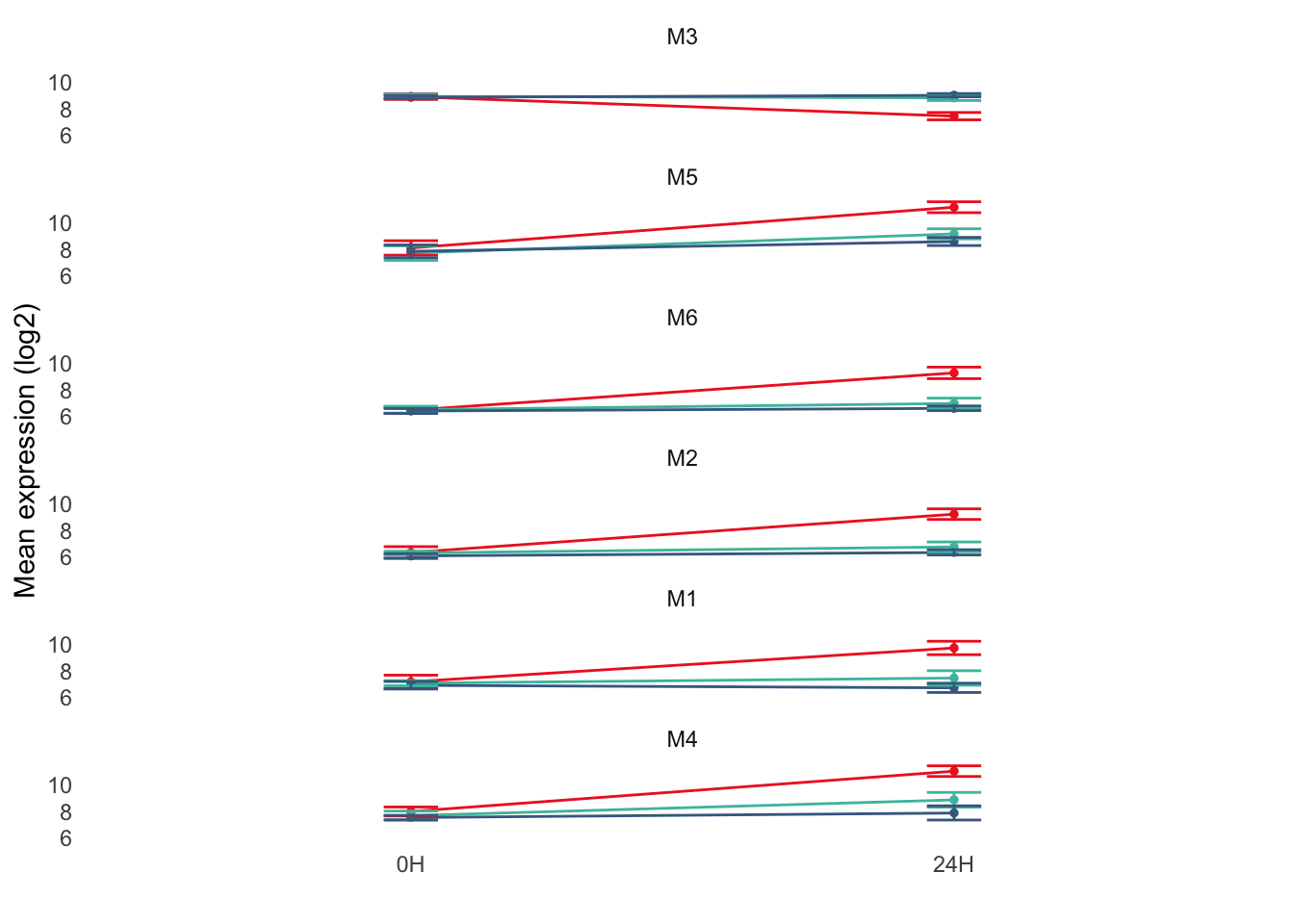
ggsave(file.path(results_dir, "modules_expression.pdf"), width = 2, height = 5)Compare DEGS across groups
# Build boolean DEG membership flags for each vaccine/group comparison.
deg_flags <- lapply(names(deg_results), function(group) {
  deg_results[[group]] %>%
    mutate(
      !!paste0("DEG_", group) := (qvalue < 0.05 & abs(logFC) > 1),         # all
      !!paste0("DEG_up_", group) := (qvalue < 0.05 & logFC > 1),           # up
      !!paste0("DEG_down_", group) := (qvalue < 0.05 & logFC < -1)         # down
    ) %>%
    dplyr::select(GeneID, starts_with("DEG_"))
})


deg_summary <- Reduce(function(x, y) full_join(x, y, by = "GeneID"), deg_flags)

deg_summary <- deg_summary %>%
  mutate(across(starts_with("DEG_"), ~tidyr::replace_na(., FALSE))) %>%
  mutate(
    DEG_class = case_when(
      DEG_mRNA & DEG_Vaxigrip & DEG_Fluad ~ "Shared by all",
      DEG_mRNA & DEG_Vaxigrip ~ "mRNA + Vaxigrip",
      DEG_mRNA & DEG_Fluad ~ "mRNA + Fluad",
      DEG_Vaxigrip & DEG_Fluad ~ "Vaxigrip + Fluad",
      DEG_mRNA ~ "mRNA only",
      DEG_Vaxigrip ~ "Vaxigrip only",
      DEG_Fluad ~ "Fluad only",
      TRUE ~ "Not DEG"
    )
  )

write.csv(deg_summary, file = file.path(results_dir, "DEG_classification.csv"), row.names = FALSE)
Upset upload
# Helper to generate UpSet plots for all/up/down DEG sets.
make_upset <- function(file_suffix) {
  # Choose columns corresponding to all, up, or down DEG flags.
  suffix <- switch(file_suffix,
                   all = "",
                   up = "_up",
                   down = "_down")
  cols <- paste0("DEG", suffix, c("_Fluad", "_Vaxigrip", "_mRNA"))
  deg_binary <- deg_summary %>%
    select(any_of(cols)) %>%
    mutate(across(everything(), ~ as.integer(as.logical(.))))
  colnames(deg_binary) <- c("Fluad", "Vaxigrip", "mRNA")
  {
  pdf(file.path(results_dir, paste0("deg_upset_", file_suffix, ".pdf")), width = 4, height = 4)
    print(
      upset(deg_binary,
            sets = c("Fluad", "Vaxigrip", "mRNA"),
            order.by = "freq", keep.order = TRUE,
            sets.bar.color = c("#49BEAA","#456990","#EE2926"),
            text.scale = 1.5)
    )
    dev.off()}
}

# Run for all / up / down
make_upset("all")
quartz_off_screen
2 make_upset("up")quartz_off_screen
2 make_upset("down")quartz_off_screen
2 Euler diagrams
make_euler <- function(file_suffix) {
  suffix <- ifelse(file_suffix == "all", "", paste0("_", file_suffix))
  deg_binary <- deg_summary %>%
    select(any_of(paste0("DEG", suffix, c("_mRNA", "_Vaxigrip", "_Fluad")))) %>%
    mutate(across(everything(), ~ as.integer(as.logical(.))))
  colnames(deg_binary) <- c("mRNA", "Vaxigrip", "Fluad")

  pdf(file.path(results_dir, paste0("deg_euler_", file_suffix, ".pdf")), width = 4, height = 4)
  print(plot(euler(deg_binary == 1),
             fills = c("#EE2926","#456990","#49BEAA"),
             labels = list(font=1),
             quantities = TRUE, edges = TRUE))
  dev.off()
}

make_euler("all")
quartz_off_screen
2 make_euler("up")quartz_off_screen
2 make_euler("down")quartz_off_screen
2 Over-representation analysis (ORA) of DEGs
gene_list_by_class <- deg_summary %>%
  filter(DEG_class != "Not DEG") %>%
  group_by(DEG_class) %>%
  summarise(genes = list(unique(GeneID))) %>%
  tibble::deframe()

ora_by_class <- setNames(lapply(names(gene_list_by_class), function(class_name) {
  genes <- gene_list_by_class[[class_name]]
  res <- tryCatch(enrichment(genes, deg_summary$GeneID), error = \(e) {
    message("Class ", class_name, ": ", e$message)
    NULL
  })
  if (!is.null(res) && nrow(res@result)) simplify(res, 0.8, "p.adjust", min) else res
}), names(gene_list_by_class))
Session info
sessionInfo()R version 4.5.3 (2026-03-11)
Platform: x86_64-apple-darwin20
Running under: macOS Sonoma 14.8.5
Matrix products: default
BLAS: /Library/Frameworks/R.framework/Versions/4.5-x86_64/Resources/lib/libRblas.0.dylib
LAPACK: /Library/Frameworks/R.framework/Versions/4.5-x86_64/Resources/lib/libRlapack.dylib; LAPACK version 3.12.1
locale:
[1] en_US.UTF-8/en_US.UTF-8/en_US.UTF-8/C/en_US.UTF-8/en_US.UTF-8
time zone: Europe/Stockholm
tzcode source: internal
attached base packages:
[1] stats4 stats graphics grDevices utils datasets methods
[8] base
other attached packages:
[1] dplyr_1.2.1 org.Mmu.eg.db_3.22.0 AnnotationDbi_1.72.0
[4] IRanges_2.43.0 S4Vectors_0.47.0 Biobase_2.69.0
[7] BiocGenerics_0.55.0 generics_0.1.4 clusterProfiler_4.18.2
[10] KEGGREST_1.49.1 pheatmap_1.0.13 eulerr_7.1.0
[13] UpSetR_1.4.0 EnhancedVolcano_1.28.2 ggrepel_0.9.8
[16] ggsci_5.0.0 gridExtra_2.3 limma_3.65.1
[19] RColorBrewer_1.1-3 gplots_3.3.0 factoextra_2.0.0
[22] ggplot2_4.0.3 matrixStats_1.5.0
loaded via a namespace (and not attached):
[1] DBI_1.3.0 bitops_1.0-9 gson_0.1.0
[4] rlang_1.2.0 magrittr_2.0.5 DOSE_4.4.0
[7] otel_0.2.0 compiler_4.5.3 RSQLite_3.52.0
[10] polylabelr_1.0.0 systemfonts_1.3.2 png_0.1-9
[13] vctrs_0.7.3 reshape2_1.4.5 stringr_1.6.0
[16] pkgconfig_2.0.3 crayon_1.5.3 fastmap_1.2.0
[19] XVector_0.49.0 labeling_0.4.3 caTools_1.18.3
[22] rmarkdown_2.31 enrichplot_1.30.3 ragg_1.5.2
[25] purrr_1.2.2 bit_4.6.0 xfun_0.57
[28] cachem_1.1.0 aplot_0.2.9 jsonlite_2.0.0
[31] blob_1.3.0 BiocParallel_1.43.4 parallel_4.5.3
[34] R6_2.6.1 stringi_1.8.7 GOSemSim_2.36.0
[37] Rcpp_1.1.1-1.1 Seqinfo_0.99.2 knitr_1.51
[40] ggtangle_0.1.2 R.utils_2.13.0 Matrix_1.7-5
[43] splines_4.5.3 igraph_2.3.1 tidyselect_1.2.1
[46] qvalue_2.42.0 rstudioapi_0.18.0 dichromat_2.0-0.1
[49] yaml_2.3.12 codetools_0.2-20 lattice_0.22-9
[52] tibble_3.3.1 plyr_1.8.9 treeio_1.33.0
[55] withr_3.0.2 S7_0.2.2 evaluate_1.0.5
[58] gridGraphics_0.5-1 polyclip_1.10-7 Biostrings_2.77.2
[61] pillar_1.11.1 ggtree_3.17.1 KernSmooth_2.23-26
[64] ggfun_0.2.0 scales_1.4.0 tidytree_0.4.7
[67] gtools_3.9.5 glue_1.8.1 lazyeval_0.2.3
[70] tools_4.5.3 data.table_1.18.4 fgsea_1.36.0
[73] fs_2.1.0 fastmatch_1.1-8 cowplot_1.2.0
[76] grid_4.5.3 tidyr_1.3.2 ape_5.8-1
[79] nlme_3.1-169 patchwork_1.3.2 cli_3.6.6
[82] rappdirs_0.3.4 textshaping_1.0.5 gtable_0.3.6
[85] R.methodsS3_1.8.2 yulab.utils_0.2.4 digest_0.6.39
[88] ggplotify_0.1.3 htmlwidgets_1.6.4 farver_2.1.2
[91] memoise_2.0.1 htmltools_0.5.9 R.oo_1.27.1
[94] lifecycle_1.0.5 httr_1.4.8 GO.db_3.22.0
[97] statmod_1.5.1 bit64_4.8.0